How to simulate groundwater levels with multiple influences ?

This example demonstrates how to simulate groundwater level varations in Rameau using multiple influences. It takes back a case study in France located near the Saint-Priest town described in two reports (82-SGN-1000-STO and 83-SGN-843-STO) and applied here with Rameau. This case study concerns groundwater level reactions due to the shutdown of a mining site.

The mine is characterized by the water level in the well named P3 and the overflow flow rate in a drainage gallery. The aquifer located near the minig site is characterized by water levels in two piezometers named A and B. The objective is to modelized groundwater level variations in A and B.

Each of these piezometers is modeled independently based on time series of :

• rainfall and PET near the site,

• water level in well P3,

• flow rate in the drainage gallery.

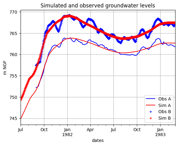
Simulations are performed on a daily basis over the period from March 1981 to February 1983 (730 days). The piezometric data from boreholes A and B and well P3, available once or twice a week, were therefore interpolated on a daily basis. The piezometric data from boreholes A and B are available for the 547-day period from the end of August 1981 to the end of February 1983. The period from March to August 1981, during which data are available, is used for initializing the model.

Simulation in the borehole A

The TOML configuration file

[files]
pet = "pet_st_priest.csv"
rainfall = "rainfall_st_priest.csv"
groundwaterobs = "gwlevel_piezo_a.csv"
groundwaterinfluence.1 = "gwlevel_well_p3.csv"
groundwaterinfluence.2 = "drainage_flow.csv"
[optimization]
maxit = 700
[watershed.all]
river.weight = 0.0
correction.pet = { value = 0.0, lower = -25, upper = 25, opti = true }
thornthwaite.capacity = { value = 50, lower = 0, upper = 250, opti = true }
progressive.capacity = { value = 0, opti = false }
transfer.halflife = { value = 0.0, opti = false }
groundwater.weight = 1.0
groundwater.observed_reservoir = 2
groundwater.storage.regression = true
groundwater.storage.coefficient = { value = 1.0, opti = true }
groundwater.base_level = { opti = true }
groundwater.1.halflife_baseflow = { value =  0.0, opti = false}
groundwater.1.halflife_drainage = { value =  20.0, opti = true, lower = 1e-2, upper = 40 }
groundwater.2.halflife_baseflow = { value =  60.0, opti = true, lower = 1e-2, upper = 150 }
influence.groundwater.1.coefficient = { value = 1.0, opti = true }
influence.groundwater.1.halflife_rise = { value = 1.5, lower = 1e-2, upper = 40, opti = true }
influence.groundwater.1.halflife_fall = { value = 10.0, lower = 1e-2, upper = 150, opti = true }
influence.groundwater.2.coefficient = { value = 1.0, opti = true }
influence.groundwater.2.halflife_rise = { value = 11.0, lower = 1e-2, upper = 40, opti = true }
influence.groundwater.2.halflife_fall = { value = 40.0, lower = 1e-2, upper = 150, opti = true }

import rameau as rm
import pandas as pd 
import matplotlib.pyplot as plt

modelA = rm.Model.from_toml("modelA.toml")
simA = modelA.run_optimization()

print(simA.get_opti_metrics('watertable'))

watersheds  Watershed 1
metrics                
nse            0.950282

Simulation in the borehole B

The TOML configuration file

[files]
pet = "pet_st_priest.csv"
rainfall = "rainfall_st_priest.csv"
groundwaterobs = "gwlevel_piezo_b.csv"
groundwaterinfluence.1 = "gwlevel_well_p3.csv"
groundwaterinfluence.2 = "drainage_flow.csv"
[optimization]
maxit = 700
[watershed.all]
river.weight = 0.0
correction.pet = { value = 0.0, lower = -25, upper = 25, opti = true }
thornthwaite.capacity = { value = 50, lower = 0, upper = 250, opti = true }
progressive.capacity = { value = 0, opti = false }
transfer.halflife = { value = 0.0, opti = false }
groundwater.weight = 1.0
groundwater.observed_reservoir = 2
groundwater.storage.regression = true
groundwater.storage.coefficient = { value = 1.0, opti = true }
groundwater.base_level = { opti = true }
groundwater.1.halflife_baseflow = { value =  0.0, opti = false}
groundwater.1.halflife_drainage = { value =  20.0, opti = true, lower = 1e-2, upper = 40 }
groundwater.2.halflife_baseflow = { value =  60.0, opti = true, lower = 1e-2, upper = 150 }
influence.groundwater.1.coefficient = { value = 1.0, opti = true }
influence.groundwater.1.halflife_rise = { value = 1.5, lower = 1e-2, upper = 40, opti = true }
influence.groundwater.1.halflife_fall = { value = 10.0, lower = 1e-2, upper = 150, opti = true }
influence.groundwater.2.coefficient = { value = 1.0, opti = true }
influence.groundwater.2.halflife_rise = { value = 11.0, lower = 1e-2, upper = 40, opti = true }
influence.groundwater.2.halflife_fall = { value = 40.0, lower = 1e-2, upper = 150, opti = true }

modelB = rm.Model.from_toml("modelB.toml")
simB = modelB.run_optimization()

print(simB.get_opti_metrics('watertable'))

watersheds  Watershed 1
metrics                
nse            0.893148

# Get the watertable simulation from optimization A
wtl_simA = simA.get_output("watertable")

# Get the watertable simulation from optimization B
wtl_simB = simB.get_output("watertable")

# Get the watertable observation
wtl_obsA = modelA.get_input("groundwaterobs")

# Get the watertable observation
wtl_obsB = modelB.get_input("groundwaterobs")

# Plot watertable
df = pd.DataFrame(
    {
        "Obs A":wtl_obsA.iloc[:, 0],
        "Sim A":wtl_simA.iloc[:, 0],
        "Obs B":wtl_obsB.iloc[:, 0],
        "Sim B":wtl_simB.iloc[:, 0],
    }
)
df.loc["1981-07-01":].plot(
    grid=True,
    title="Simulated and observed groundwater levels",
    ylabel="m NGF",
    style=["b-", "r-", "b+", "r+"]
)
plt.show()