How to simulate a groundwater level time series influenced by groundwater pumping?

This example is taken from the Gardenia tutorial [Thiéry, 2013].

This example shows how to simulate a groundwater level time series influenced by a set of pumping wells from which historical time series are known. Data from this example comes from a piezometer located near the Perpignan town and were gathered and studied by [Dagneaux, 2010] and provided by B. Ladouche and Y. Caballero from BRGM.

The following data are available:

• Daily rainfall and evapotranspiration from 1970-08-01 to 2006-07-31

• Daily piezometric levels with some gaps from 1974-02-11 to 2006-12-06.

• Monthly sum of nearby pumping well flow rates from 1998 to 2007 in m3.

Monthly time series were transformed in daily time series in order to attribute a pumping rate to each daily time step. Each monthly pumped flow rates were attributed to each day of the month, divided by the number of days in the month.

TOML configuration file

starting_date = 1999-08-01 00:00:00.000
[files]
pet = "pet.csv"
rainfall = "rainfall.csv"
groundwaterobs = "groundwaterlevel.csv"
groundwaterpumping = "groundwaterpumping.csv"
states = ""
[spinup]
starting_date = 1970-08-01 00:00:00.000
ending_date = 1999-07-31 00:00:00.000
cycles = 1
[optimization]
maxit = 450
starting_date = 1999-08-01 00:00:00.000
[watershed.all]
name = "Watershed 1"
river.weight = 0
correction.pet = { value = 0.00000, lower = -20.00000, upper = 20.00000, opti = true, sameas = 0 }
progressive.capacity = { value = 100.00000, lower = 0.00000, upper = 900.00000, opti = true, sameas = 0 }
transfer.runsee = { value = 9999.0, lower = 0.00100, upper = 9.99900E+3, opti = false, sameas = 0 }
transfer.halflife = { value = 1.00000, lower = 0.01500, upper = 20.00000, opti = true, sameas = 0 }
groundwater.weight = 1
groundwater.base_level = { opti = true }
groundwater.storage.regression = true
groundwater.storage.coefficient = { value = 100.00000, lower = 0.02000, upper = 50.00000, opti = true, sameas = 0 }
groundwater.1.halflife_baseflow = { value = 6.00000, lower = 1.50000, upper = 35.00000, opti = true, sameas = 0 }
pumping.groundwater.coefficient = { value = 1.00000, opti = true }
pumping.groundwater.halflife_rise = { value = 0.20000, lower = 0.01500, upper = 10.00000, opti = true, sameas = 0 }
pumping.groundwater.halflife_fall = { value = 1.00000, lower = 0.20000, upper = 15.00000, opti = true, sameas = 0 }

Optimization

import pandas as pd
import matplotlib.pyplot as plt
import numpy as np

import rameau as rm

# Load model from a toml file
model = rm.Model.from_toml(f"model.toml")

# Run a simulation with parameters defined in the toml file
sim = model.run_optimization()
model.tree = sim.tree

Metrics are:

# Print the groundwater level metrics
scores = sim.get_opti_metrics("watertable")
print(scores)

watersheds  Watershed 1
metrics                
nse            0.887953

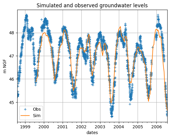
We plot groundwater level time series resulting from the optimization and we compare it with observations.

# Get the watertable simulation from optimization 1 
wtl_sim = sim.get_output("watertable")

# Get the watertable observation
wtl_obs = model.get_input("groundwaterobs")

# Plot watertable
df = pd.DataFrame(
    {
        "Obs":wtl_obs.iloc[:, 0],
        "Sim":wtl_sim.iloc[:, 0],
    }
)
df.loc["1998-08-01":"2006-07-31", :].plot(
    grid=True,
    title="Simulated and observed groundwater levels",
    ylabel="m NGF",
    style=["+", "-"]
)
plt.show() 

We plot the pulse response to an instantaneous pumped volume of $10^6$ $\mathrm{m^3}$.

sim = model.create_simulation()

data = sim._inputs.groundwaterpumping.data
data[:, :] = 0.0
data[0, :] = 1e6
sim._inputs.groundwaterpumping.data = data

data = sim._inputs.rainfall.data
data[:, :] = 0.0
sim._inputs.rainfall.data = data

data = sim._inputs.pet.data
data[:, :] = 0.0
sim._inputs.pet.data = data

sim.run(1, 200)

wt_sim = sim.get_output("watertable")
wt_sim = wt_sim.iloc[0:200].max() - wt_sim
wt_sim.iloc[0:200, :].plot(grid=True, ylabel="Groundwater level variations (m)")

<Axes: xlabel='dates', ylabel='Groundwater level variations (m)'>

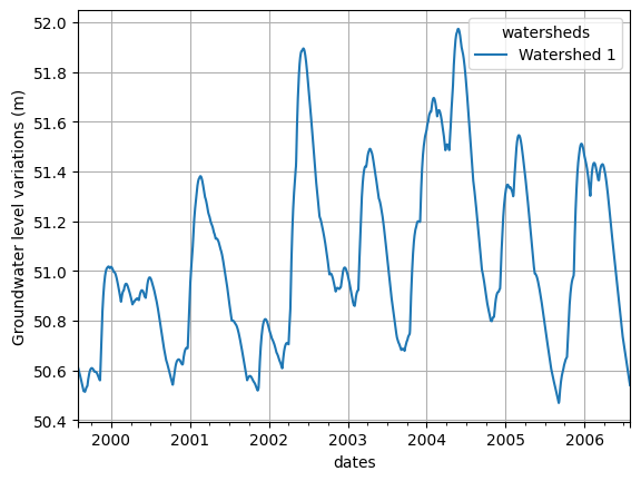
Now we plot the response to a constant pumped volume of $10^4$ $\mathrm{m^3}$.

sim = model.create_simulation()

data = sim._inputs.groundwaterpumping.data
data[:, :] = 1e4
sim._inputs.groundwaterpumping.data = data

data = sim._inputs.rainfall.data
data[:, :] = 0.0
sim._inputs.rainfall.data = data

data = sim._inputs.pet.data
data[:, :] = 0.0
sim._inputs.pet.data = data

sim.run(1, 200)

wt_sim = sim.get_output("watertable")
wt_sim = wt_sim.iloc[0:200].max() - wt_sim
wt_sim.iloc[0:200, :].plot(grid=True, ylabel="Groundwater level variations (m)")

<Axes: xlabel='dates', ylabel='Groundwater level variations (m)'>

At last we plot the influence of the rainfall alone. The amplitude of the rainfall influence is of the order of 1 me, while the amplitude of the varitions in the piezometric level is of the ordre of 6 m. The piezometer is therefore more sensitive to pumping increase than rainfall decrease.

sim = model.create_simulation()

data = sim._inputs.groundwaterpumping.data
data[:, :] = 0.0
sim._inputs.groundwaterpumping.data = data

sim.run(1, sim._ntimestep)

wt_sim = sim.get_output("watertable")
wt_sim.plot(grid=True, ylabel="Groundwater level variations (m)")

<Axes: xlabel='dates', ylabel='Groundwater level variations (m)'>