How to simulate a flash flood?

This example is taken from the Gardenia tutorial [Thiéry, 2013].

This example demonstrates the possibility of modelling flows with fine time steps. This is particularly useful for modelling floods in small catchment areas. The catchment corresponding to this example is the Patate at Durand in the Réunion Island, which covers an area of just over 10 km². The average altitude of the catchment is 977 m, ranging from 40 m at the outlet to around 1.240 m at upstream, with an average gradient of around 11%. Given these variations in altitude, it is difficult to calculate a precise water level.

This example shows the modelling of the flood resulting from the cyclone that occurs during 17-19 February 2006. For this period, we have data at 30-minute intervals of

• Estimated rainfall over the basin in mm/30 min.

• Hourly flow at the outlet, in m3/s.

No potential evapotranspiration value is available, but we have chosen a constant value of 0.1 mm/30 min, i.e. 4.8 mm/day. Each series (Rainfall, PET and river flows) covers the period from 16 to 19 February 2006, i.e. 4 days, in half-hour time steps.

TOML configuration file

Not that halflife time values are expressed in time step unit rather than in month (key unit_time_step equal to true). Flow coming from the groundwater reservoir characterized by halflife time value of 10 to 20 with 30-min time steps are not strictly speeking groundwater flows but rather delayed flow.

[files]
pet = "pet.csv"
rainfall = "rainfall.csv"
riverobs = "riverflow.csv"
[optimization]
maxit = 450
[watershed.all]
name = "Patate à Durand"
unit_time_step = true
river.area = { value = 10.00000, opti = false }
river.concentration_time = { value = 0.00000, lower = 0.00000, upper = 10.00000, opti = true, sameas = 0 }
progressive.capacity = { value = 200.00000, lower = 0.00000, upper = 650.00000, opti = true, sameas = 0 }
transfer.runsee = { value = 50.00000, lower = 1.00000, upper = 8.00000E+3, opti = true, sameas = 0 }
transfer.halflife = { value = 5.00000, lower = 0.05000, upper = 6.00000, opti = true, sameas = 0 }
groundwater.1.halflife_baseflow = { value = 10.00000, lower = 3.00000, upper = 15.00000, opti = true, sameas = 0 }
groundwater.1.halflife_drainage = { value = 6.00000, lower = 1.00000, upper = 100.00000, opti = true, sameas = 0 }
groundwater.1.exchanges = { value = 0.00000, lower = -85.00000, upper = 60.00000, opti = true, sameas = 0 }
groundwater.2.halflife_baseflow = { value = 25.00000, lower = 0.15000, upper = 50.00000, opti = true, sameas = 0 }

Optimization

import pandas as pd
import matplotlib.pyplot as plt

import rameau as rm

# Load model from a toml file
model = rm.Model.from_toml(f"model.toml")

# Run a simulation with parameters defined in the toml file
sim = model.run_optimization()

Metrics are:

# Print the riverflow metrics
scores = sim.get_metrics("riverflow")
print(scores)

watersheds     Patate à Durand
metrics                       
nse                   0.937078
kge                   0.963060
kge_2012              0.958739
nse_sqrt              0.969317
kge_sqrt              0.982956
kge_2012_sqrt         0.982059
nse_log               0.774297
kge_log               0.841491
kge_2012_log          0.835955
ratio                 1.008317

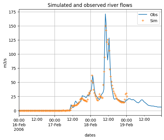
We plot river flow time series resulting from the optimization. Given the uncertainties over the actual water level in this very small catchment, it would be difficult to hope for a perfect simulation of the flood peak. It should be noted that the maximum flow is of the order of 150 m3/s, which is considerable for a small basin of around 10 km². This flash flood could not be simulated correctly with a conventional time step of 1 day, for example.

# Get the riverflow simulation
riv_sim = sim.get_output("riverflow")

# Get the riverflow observation
riv_obs = model.get_input("riverobs")

# Plot river flow
df = pd.DataFrame(
    {
        "Obs":riv_obs.iloc[:, 0],
        "Sim":riv_sim.iloc[:, 0],
    }
)
df.loc["1976-01-01":, :].plot(
    grid=True,
    title="Simulated and observed river flows",
    ylabel="m3/s",
    style=["-", "+"]
)
plt.show()