Modelling groundwater levels and river flows
This example is taken from the Gardenia tutorial [Thiéry, 2013].
This example simulates river flows and groundwater levels in a single watershed with daily observed river flows and monthly observed groundwater levels. The following data are available:
Observed daily river flow of the Selle river at Plachy from October 1989 to July 2003 (m3/s)
Observed monthly groundwater levels at Morvillers from September 1985 to July 2003 (mNGF)
Daily rainfall and potential evapotranspiration from August 1985 to July 2003 (mm/day)
The Selle River basin is a sub-basin of the Somme River basin. Its drainage area is equal to 524 km².
A simulation starts from 1989-01-01 until 2003-07-31, date of the rainfall data last record. A warmup period from 1985-01-01 to 1988-12-32 repeated three times initialize the model:
Four parameters will be optimized through bound-constrained optimization: soil water capacity, runoff/seepage partition coefficient, transfer halflife time, and baseflow halflife time.
Two will be optimized through regression: base level and groundwater storage coefficient.
Optimization of parameters uses 200 iterations at maximum and the Nash-Sutcliff coefficient as river flow metric in the objective function. Metrics are computed from 1989-01-01 to the end of the simulation (2003-07-31).
In the objective function, the weight for the river flow metric is equal to 5 and the weight for the groundwater level metric (Nash-Sutcliff coefficient) is equal to 2
TOML configuration file
starting_date = 1989-01-01
[files]
pet = "pet.csv"
rainfall = "rainfall.csv"
riverobs = "riverflow.csv"
groundwaterobs = "groundwaterlevel.csv"
[optimization]
maxit = 200
starting_date = 1989-01-01
river_objective_function = "nse"
[spinup]
starting_date = 1985-01-01
ending_date = 1988-12-31
cycles = 3
[watershed.all]
name = "Selle at Plachy"
river.weight = 5
river.area = {value=524, opti=false}
progressive.capacity = {value=180, opti=true, lower=0, upper=650}
transfer.runsee = {value=600, opti=true, sameas=0, lower=5, upper=9999}
transfer.halflife = {value=5, opti=true, sameas=0, lower=0.15, upper=25}
groundwater.weight = 2
groundwater.base_level = {value=125, opti=true}
groundwater.storage.regression = true
groundwater.storage.coefficient = {value=1, opti=true, lower=0.02, upper=50}
groundwater.1.halflife_baseflow = {value=20, opti=true, sameas=0, lower=6, upper=70}
Simulation
import pandas as pd
import matplotlib.pyplot as plt

import rameau as rm

# Load model from a toml file
model = rm.Model.from_toml(f"model.toml")

# Run a simulation with parameters defined in the toml file
sim = model.run_simulation()
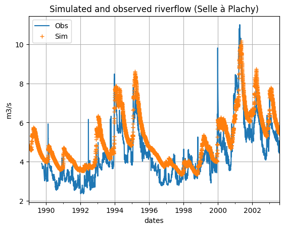
The following figure shows the observed and simulated river flow time series.
# Get the riverflow simulation
riv_sim = sim.get_output("riverflow")

# Get the riverflow observation
riv_obs = model.get_input("riverobs")

# Plot river flow
df = pd.DataFrame(
    {
        "Obs":riv_obs.iloc[:, 0],
        "Sim":riv_sim.iloc[:, 0],
    }
)
df.loc["1989-01-01":, :].plot(
    grid=True,
    title="Simulated and observed riverflow (Selle à Plachy)",
    ylabel="m3/s",
    style=["-", "+"]
)
plt.show()
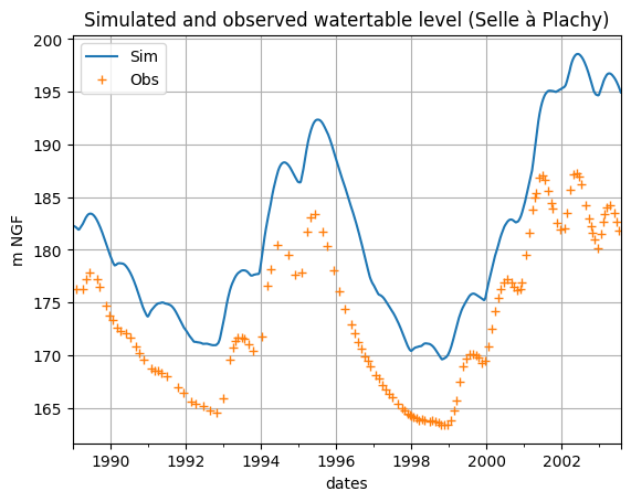
The following figure shows the observed and groundwater level time series.
# Get the watertable simulation
wtl_sim = sim.get_output("watertable")

# Get the watertable observation
wtl_obs = model.get_input("groundwaterobs")

# Plot watertable
df = pd.DataFrame({"Sim":wtl_sim.iloc[:, 0], "Obs":wtl_obs.iloc[:, 0]})
df.loc["1989-01-01":, :].plot(
    grid=True,
    title="Simulated and observed watertable level (Selle à Plachy)",
    ylabel="m NGF",
    style=['-', '+']
)
plt.show()
# Print the riverflow metrics
scores = sim.get_metrics("riverflow")
print(scores)
watersheds     Selle at Plachy
metrics
nse                   0.555237
kge                   0.808238
kge_2012              0.748022
nse_sqrt              0.528501
kge_sqrt              0.852977
kge_2012_sqrt         0.805350
nse_log               0.493272
kge_log               0.793300
kge_2012_log          0.724017
ratio                 1.166330
# Print the watertable metrics
scores = sim.get_metrics("watertable")
print(scores)
watersheds  Selle at Plachy
metrics
nse               -0.317368
Optimization
# Print the optimization settings already that have been loaded through the toml file,
# in the [optimization] section.
for key, value in model.optimization_settings.items():
    print(f'{key} = {value}')
maxit = 200
starting_date = 1989-01-01 00:00:00
ending_date = None
method = all
transformation = no
river_objective_function = nse
selected_watersheds = []
verbose = False
# Run a first optimization with the already loaded settings
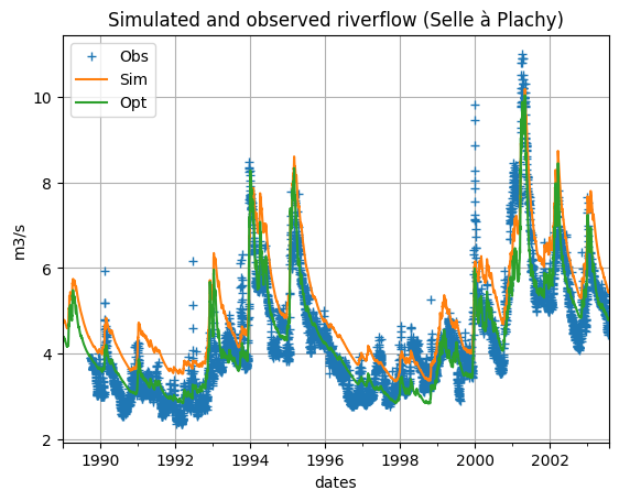
sim_opt1 = model.run_optimization()
# Get the riverflow simulation from optimization 1
riv_sim_opt1 = sim_opt1.get_output("riverflow")

# Plot river flow
df = pd.DataFrame(
    {
        "Obs":riv_obs.iloc[:, 0],
        "Sim":riv_sim.iloc[:, 0],
        "Opt":riv_sim_opt1.iloc[:, 0],
    }
)
df.loc["1989-01-01":, :].plot(
    grid=True,
    title="Simulated and observed riverflow (Selle à Plachy)",
    ylabel="m3/s",
    style=["+", "-", "-"]
)
plt.show()

# Print the riverflow optimization metrics
scores = sim_opt1.get_opti_metrics("riverflow")
print(scores)
watersheds     Selle at Plachy
metrics
nse                   0.847355
kge                   0.892512
kge_2012              0.889207
nse_sqrt              0.842473
kge_sqrt              0.894353
kge_2012_sqrt         0.891848
nse_log               0.830785
kge_log               0.888639
kge_2012_log          0.883991
ratio                 1.005227
# Get the watertable simulation from optimization 1
wtl_sim_opt1 = sim_opt1.get_output("watertable")

# Plot watertable
df = pd.DataFrame(
    {
        "Obs":wtl_obs.iloc[:, 0],
        "Sim":wtl_sim.iloc[:, 0],
        "Opt":wtl_sim_opt1.iloc[:, 0],
    }
)
df.loc["1989-01-01":, :].plot(
    grid=True,
    title="Simulated and observed watertable level (Selle à Plachy)",
    ylabel="m NGF",
    style=["+", "-", "-"]
)
plt.show()

# Print the groundwater level optimization metrics
scores = sim_opt1.get_opti_metrics("watertable")
print(scores)
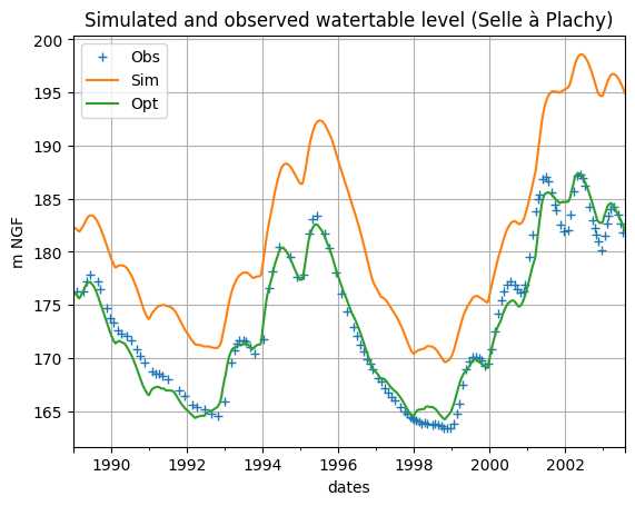
watersheds  Selle at Plachy
metrics
nse                0.970528
# Now run a second optimization but with different options
# (Gives almost the same results at the end...)
sim_opt2 = model.run_optimization(
    maxit=400,
    river_objective_function="kge_2012",
    transformation="square root"
)
# Get the riverflow simulation from optimization 2
riv_sim_opt2 = sim_opt2.get_output("riverflow")

# Plot river flow
df = pd.DataFrame(
    {
        "Obs":riv_obs.iloc[:, 0],
        "Sim":riv_sim.iloc[:, 0],
        "Opt":riv_sim_opt1.iloc[:, 0],
        "Opt 2":riv_sim_opt2.iloc[:, 0],
    }
)
df.plot(
    grid=True,
    title="Simulated and observed riverflow (Selle à Plachy)",
    ylabel="m3/s",
    style=["+", "-", "-"]
)
plt.show()

# Print the riverflow optimization metrics for optimization 2
scores = sim_opt2.get_opti_metrics("riverflow")
print(scores)
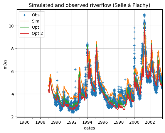
watersheds     Selle at Plachy
metrics
nse                   0.829241
kge                   0.897794
kge_2012              0.909703
nse_sqrt              0.819341
kge_sqrt              0.912902
kge_2012_sqrt         0.914578
nse_log               0.799972
kge_log               0.905674
kge_2012_log          0.898012
ratio                 0.960254
# Update the parameters of the model
model.tree = sim_opt2.tree
Forecast
# Print default options for forecast
for key, value in model.forecast_settings.items():
    print(f'{key} = {value}')
emission_date = None
scope = 1 day, 0:00:00
year_members = []
correction = no
pumping_date = None
quantiles_output = False
quantiles = [10, 20, 50, 80, 90]
norain = False
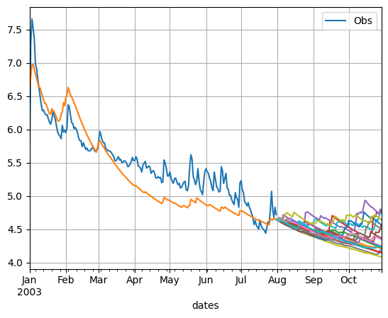
# Run a forecast with options
import datetime

sim_for = model.run_forecast(
    scope=datetime.timedelta(days=90),
)
# Now print options for forecast that have been defined for the simulation sim_for
# The default emission date corresponds to the last date of the known meteorological data
for key, value in sim_for.forecast_settings.items():
    print(f'{key} = {value}')
emission_date = 2003-07-31 00:00:00
scope = 90 days, 0:00:00
year_members = [1985, 1986, 1987, 1988, 1989, 1990, 1991, 1992, 1993, 1994, 1995, 1996, 1997, 1998, 1999, 2000, 2001, 2002]
correction = no
pumping_date = None
quantiles_output = False
quantiles = [10, 20, 50, 80, 90]
norain = False
# Get historical river flow
hist = sim_for.get_output("riverflow")

# Get forecast river flow
fore = sim_for.get_forecast_output("riverflow")

# Plot the spaghettis
riv_obs.columns = ["Obs"]
s = datetime.datetime(2003, 1, 1)
e = hist.index[-1] + sim_for.forecast_settings.scope
fig, ax = plt.subplots()
riv_obs.loc[s:e,:].plot(ax=ax)
hist.loc[s:e, :].plot(ax=ax, legend=False)
fore.loc[s:e, :].plot(ax=ax, legend=False)
ax.grid()
plt.show()
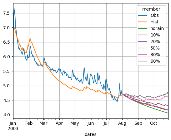
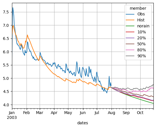
# Run a forecast with other options
sim_for = model.run_forecast(
    scope=datetime.timedelta(days=90),
    quantiles_output=True,
    norain=True
)
# Get historical river flow
hist = sim_for.get_output("riverflow")

# Get forecast river flow
fore = sim_for.get_forecast_output("riverflow")
fore = fore.xs(key="Selle at Plachy", level="watersheds", axis=1)

# Plot the spaghettis
riv_obs.columns = ["Obs"]
hist.columns = ["Hist"]
s = datetime.datetime(2003, 1, 1)
e = hist.index[-1] + sim_for.forecast_settings.scope
fig, ax = plt.subplots()
riv_obs.loc[s:e,:].plot(ax=ax)
hist.loc[s:e, :].plot(ax=ax)
fore.loc[s:e, :].plot(ax=ax)
ax.grid()
plt.show()
# Run a forecast with halflife correction.
model.tree.watersheds[0].forecast_correction.river.halflife = 30
sim_hl = model.run_forecast(
    scope=datetime.timedelta(days=90),
    quantiles_output=True,
    norain=True,
    correction="halflife"
)
# Get historical river flow
hist = sim_hl.get_output("riverflow")

# Get forecast river flow
fore = sim_hl.get_forecast_output("riverflow")
fore = fore.xs(key="Selle at Plachy", level="watersheds", axis=1)

# Plot the spaghettis
riv_obs.columns = ["Obs"]
hist.columns = ["Hist"]
s = datetime.datetime(2003, 1, 1)
e = hist.index[-1] + sim_for.forecast_settings.scope
fig, ax = plt.subplots()
riv_obs.loc[s:e,:].plot(ax=ax)
hist.loc[s:e, :].plot(ax=ax)
fore.loc[s:e, :].plot(ax=ax)
ax.grid()
plt.show()