How to simulate a threshold effect in groundwater level time series?
This example is taken from the Gardenia tutorial [Thiéry, 2013].
This example shows how to simulate groundwater level time series with overflow threshold, fractures or permeability increase near the surface, using two groundwater flow components.
The Huitrelle River basin is located in the Marne French department between the Troyes and Châlons-en-Champagne cities in the Chalk Champagne. Its drainage area at the gauging station Huitrelle at Lhuitre (H1503510) is equal to 524 km².
The Sompuis piézometer (BSS : 02255X0003) is located at about 10 km from the middle of the basin. Time series show a very marked threshold effect on the groundwater levels at an altitude of around 145 m NGF.
The following data are available:
Observed mean decadal river flow of the Huitrelle at Lhuitre from July 1997 to January 2008 (m3/s)
Observed groundwater levels at Sompuis (m NGF) from 1969 to 2008
Decadal rainfall and potential evapotranspiration from 1969 to 2008 (mm/decade)
TOML configuration file
name = "simulation"
starting_date = 1976-01-05 00:00:00.000
[files]
pet = "pet.csv"
rainfall = "rainfall.csv"
riverobs = "riverflow.csv"
groundwaterobs = "groundwaterlevel.csv"
states = ""
[input_format]
time_step = { days = 10 }
[spinup]
starting_date = 1969-01-05 00:00:00.000
ending_date = 1975-12-25 00:00:00.000
cycles = 1
[optimization]
maxit = 500
starting_date = 1976-01-05 00:00:00.000
ending_date = 2008-07-25 00:00:00.000
transformation = "square root"
[watershed.all]
name = "Huitrelle"
river.area = { value = 160.00000, opti = false }
river.concentration_time = { value = 0.00000, lower = 0.00000, upper = 10.00000, opti = true, sameas = 0 }
progressive.capacity = { value = 250.00000, lower = 0.00000, upper = 650.00000, opti = true, sameas = 0 }
transfer.runsee = { value = 20.00000, lower = 1.00000, upper = 3.00000E+3, opti = true, sameas = 0 }
transfer.halflife = { value = 4.00000, lower = 0.05000, upper = 10.00000, opti = true, sameas = 0 }
groundwater.weight = 1
groundwater.base_level = { value = 0.00000, opti = true }
groundwater.storage.regression = true
groundwater.storage.coefficient = { value = 1.00000, lower = 0.02000, upper = 50.00000, opti = true, sameas = 0 }
groundwater.1.halflife_baseflow = { value = 2.00000, lower = 0.05000, upper = 15.00000, opti = true, sameas = 0 }
Optimization without threshold
import pandas as pd
import matplotlib.pyplot as plt

import rameau as rm

# Load model from a toml file
model = rm.Model.from_toml(f"model.toml")

# Run a simulation with parameters defined in the toml file
sim = model.run_optimization()
Optimized parameters are:
w = sim.tree.watersheds[0]
print("Base level = ", round(w.groundwater.base_level.value, 4), " m NGF")
print("Storage coefficient = ", round(w.groundwater.storage.coefficient.value, 4), " %")
Base level =  132.0037  m NGF
Storage coefficient =  0.0979  %
Metrics are a priori correct:
# Print the riverflow metrics
scores = sim.get_metrics("riverflow")
print(scores)
watersheds     Huitrelle
metrics
nse             0.922140
kge             0.952668
kge_2012        0.950767
nse_sqrt        0.907357
kge_sqrt        0.951250
kge_2012_sqrt   0.951697
nse_log         0.865834
kge_log         0.855846
kge_2012_log    0.814282
ratio           0.974457
# Print the watertable metrics
scores = sim.get_metrics("watertable")
print(scores)
watersheds  Huitrelle
metrics
nse          0.824961
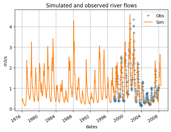
We plot river flows and groundwater levels time series from this first optimization.
# Get the riverflow simulation
riv_sim = sim.get_output("riverflow")

# Get the riverflow observation
riv_obs = model.get_input("riverobs")

# Plot river flow
df = pd.DataFrame(
    {
        "Obs":riv_obs.iloc[:, 0],
        "Sim":riv_sim.iloc[:, 0],
    }
)
df.loc["1976-01-01":, :].plot(
    grid=True,
    title="Simulated and observed river flows",
    ylabel="m3/s",
    style=["-", "+"]
)
plt.show()
# Get the watertable simulation
wtl_sim = sim.get_output("watertable")

# Get the watertable observation
wtl_obs = model.get_input("groundwaterobs")

# Plot watertable
df = pd.DataFrame({"Sim":wtl_sim.iloc[:, 0], "Obs":wtl_obs.iloc[:, 0]})
df.loc["1976-01-01":, :].plot(
    grid=True,
    title="Simulated and observed groundwater levels",
    ylabel="m NGF",
    style=['-', '+']
)
plt.show()
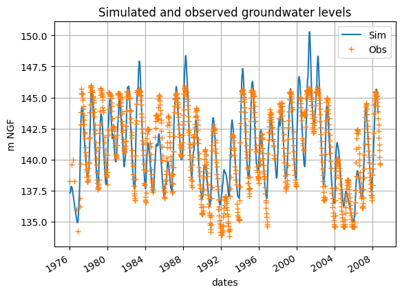
This plot shows that the simulated groundwater levels exeed the observed maximal level of around 145 m NGF (1983, 1988, 1994, 2001). We propose to perform a second optimization run by letting the possibility for the model to have an overflow threshold corresponding approximatively to this 145 m NGF value.
Optimization with groundwater threshold
This is exactly the same configuration but now by introducting a threshold in the groundwater reservoir, i.e. a flow that appears only if the groundwater reservoir level exceeds a threshold value.
The overflow threshold value corresponding to the 145 m NGF is deduced as follows:
\(H_o = (145 - H_b)S\)
\(H_o = (145 - 132.0037) \times 0.000979 = 12.7 \times 10^{-3} \ \mathrm{mNGF} = 12.7 \ \mathrm{ mm}\)
We modify the model to start from this value during the optimization. The initial value for the overflow halflife time is set to 0.2 months. This quick value allows to limit the rising of groundwater levels.
# Run a seoncd optimization with optimization threshold parameters now optimized
model.tree.watersheds[0].groundwater.reservoirs[0].overflow.threshold = rm.Parameter(
    value = 12.7, lower=0.0, upper=500, opti=True
)
model.tree.watersheds[0].groundwater.reservoirs[0].overflow.halflife = rm.Parameter(
    value = 0.2, lower=0.05, upper=15, opti=True
)
sim = model.run_optimization()
Optimized parameters are:
w = sim.tree.watersheds[0]
print("Base level = ", round(w.groundwater.base_level.value, 4), " m NGF")
print("Storage coefficient = ", round(w.groundwater.storage.coefficient.value, 4), " %")
print("Overflow threshold = ", round(w.groundwater.reservoirs[0].overflow.threshold.value, 4), " mm")
print("Overflow halflife time = ", round(w.groundwater.reservoirs[0].overflow.halflife.value, 4), " mm")
Base level =  129.9167  m NGF
Storage coefficient =  0.0884  %
Overflow threshold =  13.2153  mm
Overflow halflife time =  0.2967  mm
Metrics for river flow stays correct while metrcis for grondwater levels are improved:
# Print the riverflow metrics
scores = sim.get_metrics("riverflow")
print(scores)
watersheds     Huitrelle
metrics
nse             0.917490
kge             0.921584
kge_2012        0.916206
nse_sqrt        0.901556
kge_sqrt        0.939153
kge_2012_sqrt   0.941131
nse_log         0.858213
kge_log         0.665817
kge_2012_log    0.581947
ratio           0.936956
# Print the watertable metrics
scores = sim.get_metrics("watertable")
print(scores)
watersheds  Huitrelle
metrics
nse          0.880018
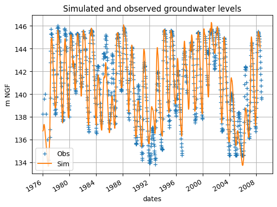
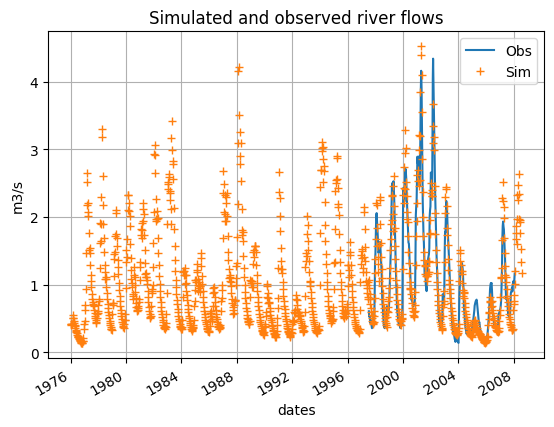
We plot river flows and groundwater level time series. As expected the simulated groundwater levels do not exceed the threshold value noted in the observations.
# Get the riverflow simulation from optimization 1
riv_sim = sim.get_output("riverflow")

# Plot river flow
df = pd.DataFrame(
    {
        "Obs":riv_obs.iloc[:, 0],
        "Sim":riv_sim.iloc[:, 0],
    }
)
df.loc["1976-01-01":, :].plot(
    grid=True,
    title="Simulated and observed river flows",
    ylabel="m3/s",
    style=["+", "-", "-"]
)
plt.show()
# Get the watertable simulation from optimization 1
wtl_sim = sim.get_output("watertable")

# Plot watertable
df = pd.DataFrame(
    {
        "Obs":wtl_obs.iloc[:, 0],
        "Sim":wtl_sim.iloc[:, 0],
    }
)
df.loc["1976-01-01":, :].plot(
    grid=True,
    title="Simulated and observed groundwater levels",
    ylabel="m NGF",
    style=["+", "-", "-"]
)
plt.show()